Real-Time Magnetic Monopole Interaction Simulation
Summary
This python code is a simulation of how a hypothetical magnetically charged particle (magnetic monopole) would interact with and move near electrically charged particles (more information can be found at https://en.wikipedia.org/wiki/Magnetic_monopole). As many particles as desired can be added along with their initial conditions and the program will output a 3D simulation of their motions.
Purpose
I created this because my physics teacher introduced me to this hypothetical concept of magnetic monopoles, and I was very interested in seeing how they would behave if they were real. Since orbital mechanics are difficult to solve by hand and often don’t have closed solutions, I tried to find a simulation of magnetic monopoles online but I couldn’t find what I was looking for. I created this so that I could see for myself the motions of these particles.
Technologies Used
- Python: Core programming language for calculations and logic.
- Matplotlib: Used for plotting the real-time graph of particle distances.
- NumPy: Used for numerical computations.
- PyCharm: Used free version for students for coding and running.
Model
I assumed that the particles are moving at slow enough speeds that the electric and magnetic fields are coulombic (spherically symmetric, proportional to 1/r^2). The electric field and magnetic fields produced by a particle with electric charge q and magnetic charge b are given by
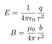
and for convenience I chose the constant coefficients in front of the charge over distance squared terms to be equal to 1 (this also makes the speed of light equal to 1). I calculated the fields produced by each of the charges and used that to find the force on each charge using the Lorentz Force equation with magnetic charge added given by
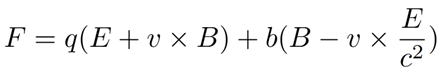
I then used a version of Newton’s method with a time step of t=0.01 to calculate the velocity and position over time of each particle. The time step can be changed in the variable called tim, however lowering it will cause the simulation to take longer to run.
How to Run
There is a section labeled in the code where the particles are created (with a few examples given) along with instructions. The code will create a separate matplotlib window when run with the simulation unless the last few lines are uncommented to save as a gif.
Implementation
Code Structure
The program is structured into classes and functions:
- Particle Class: Encapsulates particle properties and calculates acceleration due to electromagnetic forces.
- Field Calculations: Updates electric and magnetic fields based on particle locations.
- Animation: Visualizes the particles' trajectories in a 3D space.
Simulation Parameters
- Time step (Δt): 0.01 s
- Initial particle properties (mass, charges, position, velocity)
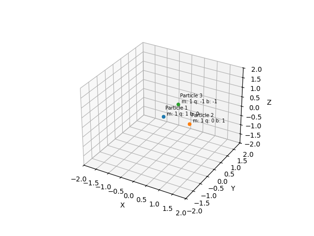
- Space constraints: [-2, 2] for x, y, z axes
Visualization
A 3D scatter plot displays particles, and labels show the properties of each particle.
Appendix: Code Listing
import numpy as np
import math
import matplotlib
matplotlib.use('TkAgg')
import matplotlib.pyplot as plt
import matplotlib.animation as animation

class particle:
    epsilon=1/(4*math.pi)
    mu=4*math.pi
    def __init__(self,mass,electricCharge,magneticCharge,position,velocity,electricField=np.array([0,0,0]),magneticField=np.array([0,0,0])):
        self.mass=mass
        self.electricCharge=electricCharge
        self.magneticCharge=magneticCharge
        self.position=position
        self.velocity=velocity
        self.electricField=electricField
        self.magneticField=magneticField
    def acceleration(self):
        force=self.electricCharge*(self.electricField+np.cross(self.velocity,self.magneticField))+self.magneticCharge*(self.magneticField-np.cross(self.velocity,self.electricField)/(particle.epsilon*particle.mu))
        acceleration=force/self.mass
        return acceleration

tim=0.01
particleList=[]

# List Of Particles (Properties in order are mass, electric charge, magnetic charge, position, velocity within the particle function)
particleList.append(particle(1,1,0,np.array([0,0,0]),np.array([0,0,0])))
particleList.append(particle(1,0,1,np.array([1,0,0]),np.array([0,1,0])))
particleList.append(particle(1,-1,-1,np.array([0,1,0]),np.array([0.5,0,0])))

fig = plt.figure(num="Electric and Magnetic Charge Simulation")
ax = fig.add_subplot(111,projection='3d')
ax.set_xlim([-2,2])
ax.set_ylim([-2,2])
ax.set_zlim([-2,2])
ax.set_xlabel('X')
ax.set_ylabel('Y')
ax.set_zlabel('Z')

# Field Updating
def animate(i):
    ax.clear()
    ax.set_xlim([-2, 2])
    ax.set_ylim([-2, 2])
    ax.set_zlim([-2, 2])
    ax.set_xlabel('X')
    ax.set_ylabel('Y')
    ax.set_zlabel('Z')
    for particle1 in particleList:
        particle1.electricField=np.array([0,0,0])
        particle1.magneticField=np.array([0,0,0])
        for particle2 in particleList:
            if particle2 is not particle1:
                displacement=particle1.position-particle2.position
                if np.dot(displacement,displacement) == 0:
                    continue
                eField=1/(4*math.pi*particle.epsilon)*(particle2.electricCharge)/np.dot(displacement,displacement)*displacement/np.linalg.norm(displacement)
                mField=particle.mu/(4*math.pi)*(particle2.magneticCharge)/np.dot(displacement,displacement)*displacement/np.linalg.norm(displacement)
                particle1.electricField=particle1.electricField+eField
                particle1.magneticField=particle1.magneticField+mField
    for particle1 in particleList:
        a=particle1.acceleration()
        particle1.position = particle1.position + tim * particle1.velocity + tim ** 2 * a
        particle1.velocity= particle1.velocity + tim * a
    for particle1 in particleList:
        i=particleList.index(particle1)
        ax.scatter(particle1.position[0],particle1.position[1],particle1.position[2], s=20)
        ax.text(particle1.position[0]+0.05,particle1.position[1]+0.05,particle1.position[2]+0.05, "Particle " + str(i+1) + "\n m: " + str(particle1.mass) + " q: " + str(particle1.electricCharge) + " b: " + str(particle1.magneticCharge), fontsize =7)

ani = animation.FuncAnimation(fig, animate, frames=400, interval=1, blit=False)

# For saving the animation as gif, uncomment two lines below and change the directory
# writer = animation.PillowWriter(fps=30, metadata=dict(artist='Cyan Gupta'), bitrate=1800)
# ani.save('../../../Downloads/Animation.gif', writer=writer)
plt.show()